cs7641_census_project
Predicting Election Flips from Changes in Census Data
Introduction
In recent years, there has been a socio-political shift in rural and urban areas which has resulted in greater divides at the local and national level. Our project aims to model economic, demographic, and social changes at a county level to predict the potential course of future elections, so we can discern the major factors that contribute to political divide.
Problem Definition
Given data collected by the US Census Bureau [1], we want to understand the influence that shifts in demographic, economic, and social factors have on the political scene, and if forecasting future outcomes [2-4] can be accomplished using a machine learning model. The current state-of-the-art looks at a relatively limited set of features, leaving many potentially useful variables unexplored. Our proposed solution will accommodate a large number of Census data attributes to gain a deeper understanding of the context using a series of unsupervised and supervised techniques.
We define our supervised learning task as a binary classification task, in which we predict whether or not the winning party for a particular county (Democrat or Republican) flips for a particular election. We define a positive as a “flip”.
Data
Census Data
Our dataset consists of a large set of different datasets, each of which captures a different statistical measure. For this project, we have included features from the following datasets:
- Census Bureau American Community Survey (ACS): 5-Year Estimates [5]
- Community Business Patterns (CBP) [6]
- ACS Migration Flows (AMF): 5-Year Estimates [7]
The ACS covers a broad range of variables regarding social, economic, demographic, and housing information across geographical areas in the United States. On an annual basis, comprehensive 5-Year Estimates are released for the five years leading up to that year. We utilize 175 unique variables from their Data Profile tables:
- 21 social variables (related to education, school enrollment, and fertility rate)
- 45 economic variables (related to employment, income, occupation, industry, and poverty)
- 32 housing variables (related to occupancy, housing value, and owner/renter costs)
- 67 demographic variables (related to race, ethnicity, nationality, gender, and age)
CBP provides subnational economic data by industry on an annual basis. From this dataset, we get four variables: first quarter payroll, annual payroll, number of employees, and number of establishments.
AMF provides period estimates that measure change in residence. From this dataset, we get six variables.
We used a series of Census API keys to pull data for each of the Census datasets into a CSV format, and we have included a script to download and collate the data. The primary keys for each dataset are:
- YEAR
- STATE
- COUNTY
Every data record has a unique combination of these keys, and the year generally varies from 2009 to 2019 (inclusive), the time range of data we were able to obtain from the census website. The state and county are two designated numeric identifiers, known as FIPS codes. A state is denoted by two digits, and a county is denoted by three digits, together forming a unique five-digit FIPS code. The census data is available for all counties in all states.
Election Data
We pull county-level data for presidential and senatorial races for the years within the range of available Census data; specifically, the 2012 and 2016 presidential elections, and all senatorial races from 2012 to 2018. This data is publicly available from Dave Leip’s Atlas of U.S. Elections [[8]]. We implemented a script that utilizes Selenium, a browser automator software, to automatically browse pages on the site using URL and use HTML information to pull the data into .csv files. The results, available for each county for a given election year, serve as the basis for our labels.
Data handling
- We removed categorical features, as encoding categorical features would have increased the dimensionality of the data.
- We removed linearly dependent features, as they would not be useful for our model.
- We used Random Forest Regression to impute features with missing data. If a feature had more than 20% missing data, it was removed. By doing this, we reduced the dimensionality of our data from an original amount of 200 to 175 features, out of which 10 needed to be imputed.
- We normalized the data, to reduce the variance of the data.
- We constructed dataloaders to handle all preprocessing and feature extraction. For different models, we employed different feature extraction approaches - see the figure below.
- Finally, we merged the election results with the Census Data using an inner join on the aforementioned three primary keys.

Final dataset statistics
| Data points (county/state/year) | Positive labels | Non-positive labels | |
|---|---|---|---|
| Presidential data | 5860 | 509 | 5351 |
| Senatorial data | 7434 | 1234 | 6200 |
Methods
Unsupervised learning (PCA for dimensionality reduction)
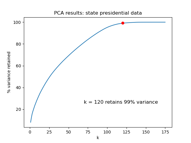
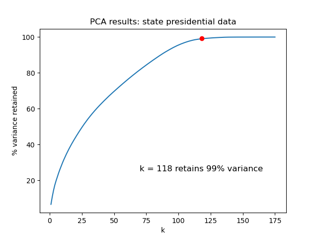
After preprocessing the data, we implemented Principal Component Analysis (PCA) for identifying the most important principal components, and aimed to retain 99% variance. By using PCA, we reduced the dimensionality of the dataset, while observing which features are the most desirable for a model predicting election results. We implemented PCA using the scikit-learn library. Results and selected values of k are shown in plots in the “Results” section.
Supervised learning
For classification, we utilized three scikit-learn models, along with an ensemble model that combines the three. These models are designed to take in the vectors from PCA, generated from one-year changes of the raw census variables. The models are:
- AdaBoostClassifier
- RandomForestClassifier
- BaggingClassifier
In addition to the above models, we implemented a recurrent neural network (RNN) using Keras. The model is designed to take in sequences of length 3, representing the cumulative change in the raw census variables for the three years leading up to an election year.
SMOTE: addressing the class imbalance
For all the above approaches, in order to address the large class imbalance in our data, we utilized a SMOTE [9] over-sampler to create synthetic data of the minority class in order to create a class balance of 1 in our training data. In addition, we use an undersampler to reduce the number of samples in the majority class. Both are from the Python library imblearn.
Hyperparameters
We performed hyperparameter tuning for each of the models, and arrived at the following values:
- For AdaBoost, we set the number of estimators to 90.
- For random forest, we set the number of trees to 1500.
- For bagging, we set the number of estimators to 50.
- With the aforementioned exceptions, we use the default hyperparameters for the sklearn models.
- For RNN, we use a dropout of 0.2, a batch size of 128, Adam optimizer, and trained for 10 epochs.
- All models used a 80-20 train-test split.
Results
PCA
| PCA results: presidential data | PCA results: senatorial data |
|---|---|
 |
 |
Supervised learning (Ensemble model)
This table shows the F1 scores of each model for each dataset:
| AdaBoost | Random Forest | Bagging | Ensemble | RNN | |
|---|---|---|---|---|---|
| Presidential data | 0.179 | 0.112 | 0.167 | 0.118 | 0.456 |
| Senatatorial data | 0.350 | 0.258 | 0.267 | 0.284 | 0.476 |
The following are confusion matrices that correspond to the F1-scores for AdaBoost:
AdaBoost for Presidential:
| Non-flip | Flip | |
|---|---|---|
| Non-flip | 838 | 234 |
| Flip | 68 | 33 |
AdaBoost for Senatorial:
| Non-flip | Flip | |
|---|---|---|
| Non-flip | 988 | 518 |
| Flip | 176 | 187 |
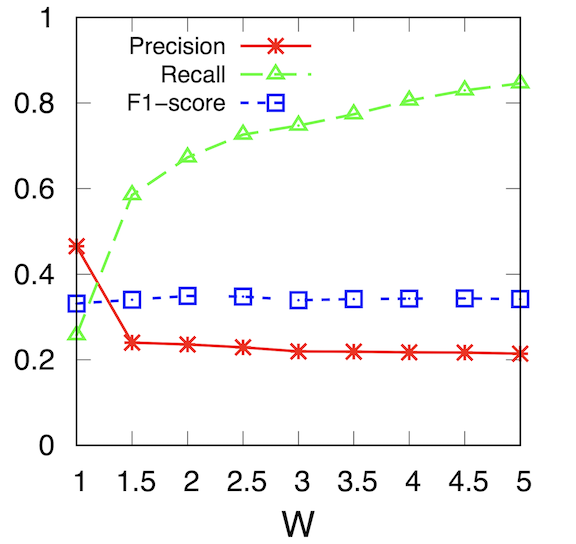
The following is a plot representing the degree to which the F1-score, precision, and recall vary with the AdaBoost Senatorial classifier. The variable W represents the ratio to which the minority class (“Flip”) is prioritized over the majority class (“Non-flip”) at the time of training / parameter learning. We decided to vary this value in order to explore whether or not modifying it would contribute to improving performance in the face of class imbalance.
Discussion
One of our key observations is the drastic improvement in performance of the RNN vs the sklearn models. We believe this is because the data that we pass into RNN is more information-rich than that which we pass into the sklearn models. Specifically, we use a sequence of yearly changes over three years prior to an election for the RNN instead of a change over a single year for the sklearn models. This allows us to capture more detailed information about how certain economic, demographic, etc. variables of a particular county has changed over the election-relevant period.
Another one of our key observations is that the presidential models consistently performed worse than the senatorial models. We hypothesize that this is because presidential races are more strongly influenced by attitudes of political partisanship, information that the Census data cannot encode. In addition, senate races are state-level while presidential races are national-level, possibly suggesting that the candidate’s proximity to home has an added effect as well.
Out of the sklearn models, AdaBoost performed the best for both the presidential and senatorial data. We believe this is because AdaBoost is more robust to the curse of dimensionality than the other models, allowing it to perform better on high-dimensional data.
In addition, according to the plot, the F1-score stays roughly the same as the training weight of the minority class increases, buoyed by a gradual increase in recall but a gradual decrease in precision. In other words, it is more likely to classify minority class samples correctly, but at the cost of classifying majority class samples incorrectly. This leads us to conclude that altering this variable did not have a significant effect in improving the performance of the classifier.
Moreover, we make the following broad, general observations:
- Lack of real-world samples in the minority class. In real-world elections, only a small handful of elections see power transferred from one party to another. This creates a large, but natural, imbalance in the dataset that we observe even SMOTE can only partially correct. This class imbalance is a major factor on our F1-score results, which are low for a classification task.
- Lack of samples in general. Our dataset is limited by the bottleneck of the availability of the Census ACS data. The 5-year figures only date by to 2009, which explains why we could not generate features for elections before 2012 (our longest range approach requires a three-year sequence of census data). With more data dating further back, we would expect the classification result to improve.
- Curse of dimensionality. We used either 118 or 120 PCA-created columns as our features for the sklearn models, which we believe may still be too many to make distances between points in Euclidean space be meaningful. This could explain the poor classification performance for many of the models.
- Construction of the labels. By defining our label as a binary classification, we cannot fully grasp changes with high enough granularity to make changes in the input features meaningful. It could also be useful to consider this task from a regression perspective instead of purely a classification one.
Conclusions
We were able to successfully produce at least one classifier that could do a decent job at predicting whether or not a county would flip in a presidential or senatorial election. This demonstrates that the census features that we selected can provide a measurable amount of information about when that might happen.
For future work:
- We can continue to explore RNN-based approaches, since based on our results, that approach shows the most promise.
- We can also continue to find datasets to produce data points for earlier years in order to expand our training set. We also do not have to limit ourselves to the United States; we can explore similar census data from other countries (specifically democracies) too.
- We can try to alter our problem from a classification task to a regression task.
Video Proposal
https://github.com/V-TERM/cs7641_census_project/blob/668bfdc1adaf488440158ca84231d255c03efdf6/Project_Proposal.mp4
References
[1] United States Census. “Explore Census Data.” Retrieved from https://data.census.gov/cedsci/.
[2] Caballero, Michael. “Predicting the 2020 US Presidential Election with Twitter.” arXiv preprint arXiv:2107.09640 (2021). Retrieved from https://arxiv.org/abs/2107.09640.
[3] Colladon, Andrea Fronzetti. “Forecasting election results by studying brand importance in online news.” International Journal of Forecasting 36.2 (2020): 414-427. Retrieved from https://arxiv.org/abs/2105.05762.
[4] Sethi, Rajiv, et al. “Models, Markets, and the Forecasting of Elections.” arXiv preprint arXiv:2102.04936 (2021). Retrieved from https://arxiv.org/abs/2102.04936.
[5] United States Census. “American Community Survey 5-Year Data (2009-2019).” Retrieved from https://www.census.gov/data/developers/data-sets/acs-5year.html.
[6] United States Census. “County Business Patterns (CBP).” Retrieved from https://www.census.gov/programs-surveys/cbp.html.
[7] United States Census. “American Community Survey Migration Flows.” Retrieved from https://www.census.gov/data/developers/data-sets/acs-migration-flows.html.
[8] Dave Leip’s Atlas of U.S. Elections. “United States Presidential Election Results.” Retreived from https://uselectionatlas.org/RESULTS/.
[9] Brownlee, Jason. “SMOTE for Imbalanced Classification with Python.” Retrieved from https://machinelearningmastery.com/smote-oversampling-for-imbalanced-classification/